Home » Assignments
Category Archives: Assignments
Assignment 3
Nonstandard Normal Distributions
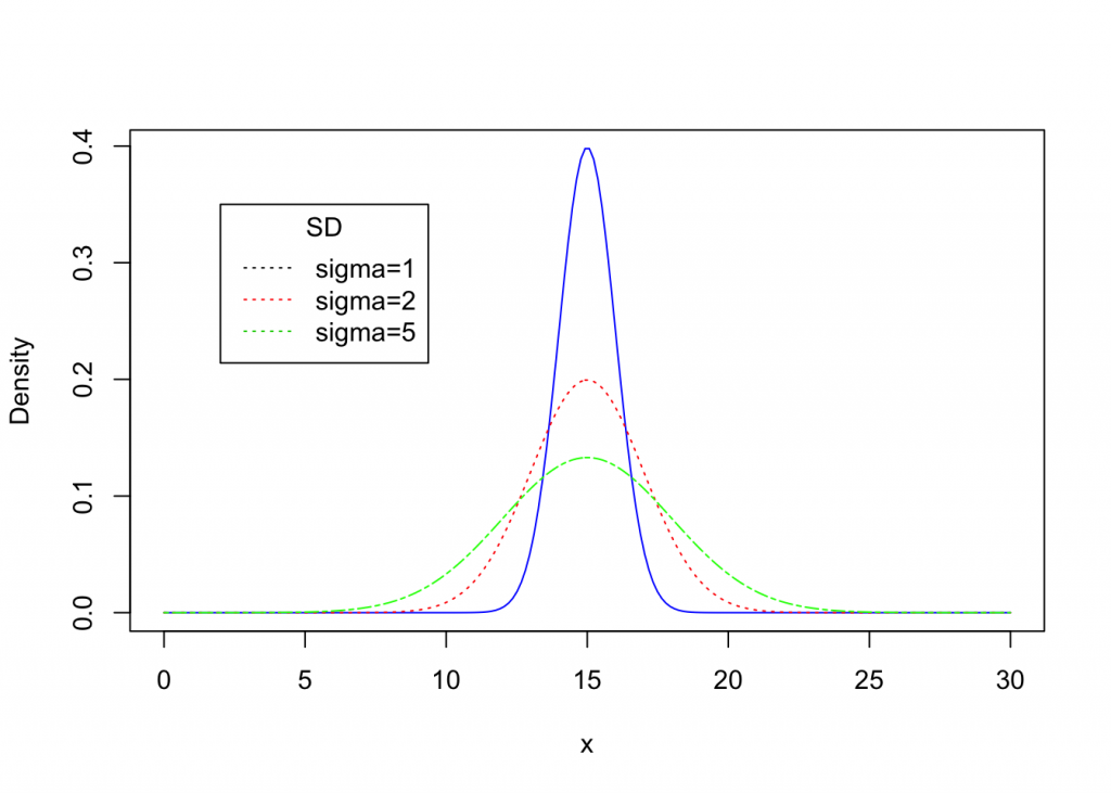
Here are nonstandard density curves with a mean equal to 15 and various standard deviations.
Model Problem1
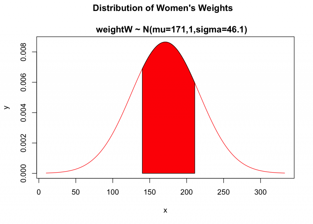
U.S. Air Force once used ACES-II ejection seats designed for men weighing between 140 lb and 211 lb. Given that women’s weights are normally distributed with a mean 171.1 lb and a standard deviation of 46.1 lb (based on data from the National Health Survey), what percentage of women have weights that are within those limits? Were many excluded from those past specifications?
Model Solution when Using z-tables
Given: Distribution Statement: heightW ~ N(mean = 171.1lb.,sd = 46.1lb.) and heightW boundaries: 140lb and 211lb
Objective(s): a. The proportion of women’s heights within the boundaries.
b. Were many women excluded from those past specifications?
Solution Plan
1. We will sketch and label nonstandard distribution of women’s heights, (heightW) and include distribution statement as its title.
2. Next, we will calculate z-scores for the boundaries and determine the area under density cure within these limits.
3. Finally, we will provide a written statement regarding obtained results.
1. Solution
Lower boundary: x=140
Upper boundary: x=211
2. Model solution when using z-tables
Now we will convert boundaries x=140 and x=211 to respective z-scores:
x = 140 corresponds to z = -0.67
x = 211 corresponds to z = 0.84
The area under the density curve within the limits is found from z-table it is equal to 0.5564. The cumulative area under both tails is 1 – 0.5564=0.4436
3. Statements about obtained results
3a. Just about 55.64% of women met past weight requirements.
3b. About 44.00% of women were excluded from past weight specifications.
Model Solution when Using R for Calculations
For part a. we will use: pnorm(x,mean,sd) code in the following way:
pnorm(211, mean=171.1, sd=46.1)-pnorm(140,mean=171.1, sd=46.1)## [1] 0.556662For part b we will use: code, 1- the previous answer:
1-0.556662## [1] 0.443338However, we may use more fancy code, (cut/paste) as follow:
1 -(pnorm(210, mean=171.1, sd=46.1)-pnorm(140,mean=171.1, sd=46.1))## [1] 0.4493441Assignment 3
Extra Credit: #29 and #33 from page: 252-253. Note: Follow model solution, part; (1), (2), and (3) in order to obtain full credit.
Extracted from M.F Triola, Essential s of Statistics Sixth Edition, Pearson. Essentials of Statistics page: 252, #27↩
- Extracted from M.F Triola, Essential s of Statistics Sixth Edition, Pearson. Essentials of Statistics page: 252, #27↩
Assignment 2
The Normal Distribution
Here is the Standard Normal Distribution Density Curve is also known as the Bell Curve.
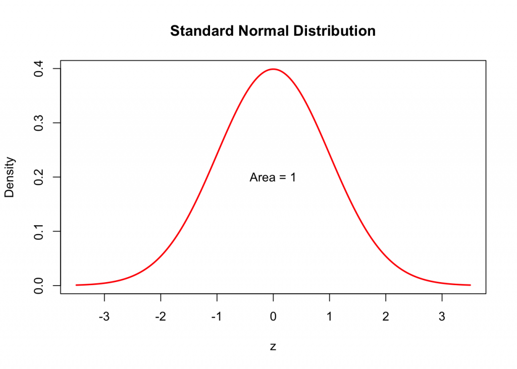
How do we find the area under the Standard Normal Density Curve?
Example 1
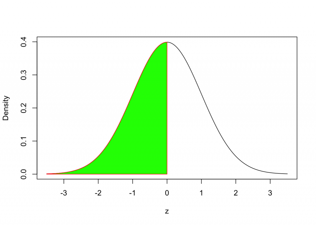
We will use the following syntax:
pnorm(0,mean=0,sd=1)## [1] 0.5Example 2
How do we find the area under the Standard Normal Density Curve to the left of z = 1.25?
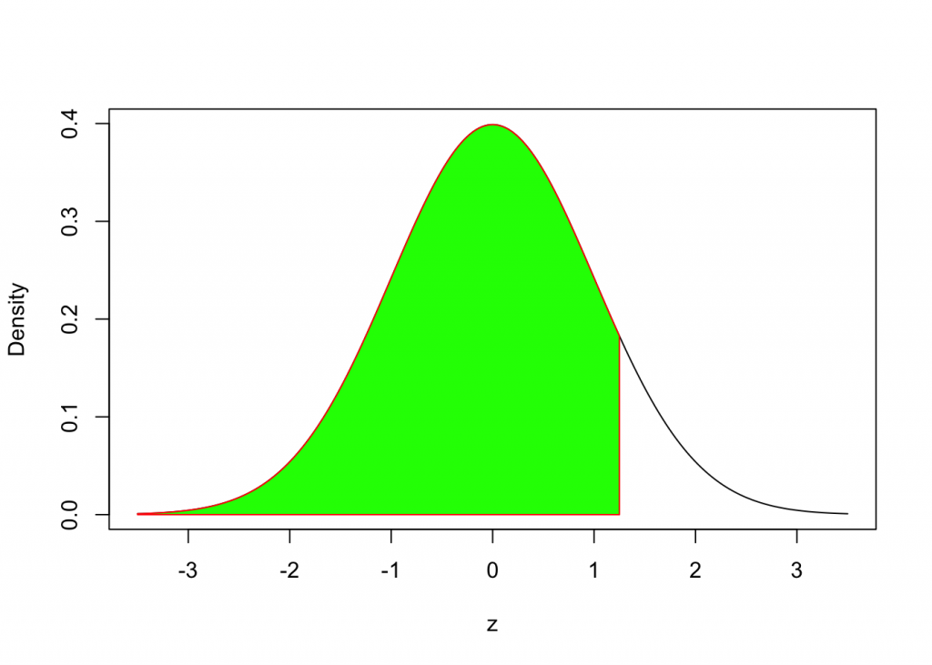
pnorm(1.25, mean=0,sd=1)## [1] 0.8943502Example 3
How do we find the area under the Standard Normal Density Curve to the right of z = 1.5?
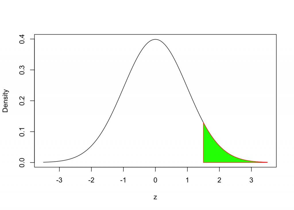
We can use the following syntax:
1 - pnorm(1.5, mean=0, sd=1)## [1] 0.0668072Alternatively the code below
pnorm(1.5, mean=0, sd = 1, lower.tail = FALSE)## [1] 0.0668072Example 4
How do we determine the area under the Standard Normal Curve between two z-values, (eg. z = -1.25 and z = 1.25)?
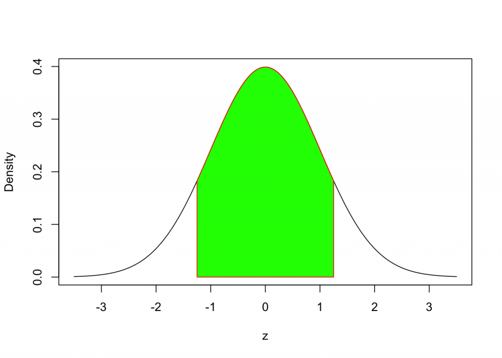
We can calculate the difference of two areas as follows:
pnorm(1.25, mean = 0, sd = 1) - pnorm(-1.25, mean = 0, sd = 1)## [1] 0.7887005Summary:
The following code pnorm(z, mean, sd) provides the area under the Standard Normal Density Curve to the left of z-value.
Assignment 2
The bone density test scores follow standard normal distribution for children, healthy premenopausal young women, and men under 50. Assume that a randomly selected person is subjected to a bone density test. Find the probability that this person has a score:
- z < -2.5
- -2.5 < z < -1
- z > -1.
Note: For each part: a, b and c include distribution statement, density curve with shaded area. Also, use a full and complete sentence as the answer to a, b, and c part.
link
Assignment 1
Tutorial/Extra Credit Assignment
How to partition Births Data Set1 by gender?
How to create a histogram of Birth Weight Data Set for each gender?
Upload data set by using the following syntax:
BirthsD <-read.csv(file.choose(),header =TRUE)
attach(BirthsD)
head(BirthsD,3)
## FACILITY INSURANCE GENDER..1.M.
## 1 Albany Medical Center Hospital Insurance Company 0
## 2 Albany Medical Center Hospital Blue Cross 1
## 3 Albany Medical Center Hospital Blue Cross 0
## LENGTH.OF.STAY ADMITTED DISCHARGED BIRTH.WEIGHT TOTAL.CHARGES
## 1 2 FRI SUN 3500 13985.7
## 2 2 FRI SUN 3900 3632.5
## 3 36 WED THU 800 359091.0Select all rows from the BirthsD data set that pertain to girls’ births and include all variables, (columns).
Start by naming this subset girlD, (girls data).
girlD <-BirthsD[GENDER..1.M. == "0",]
attach(girlD)
## The following objects are masked from BirthsD:
##
## ADMITTED, BIRTH.WEIGHT, DISCHARGED, FACILITY, GENDER..1.M.,
## INSURANCE, LENGTH.OF.STAY, TOTAL.CHARGEShead(girlD)## FACILITY INSURANCE GENDER..1.M.
## 1 Albany Medical Center Hospital Insurance Company 0
## 3 Albany Medical Center Hospital Blue Cross 0
## 6 Albany Medical Center Hospital Blue Cross 0
## 7 Albany Medical Center Hospital Medicaid 0
## 9 Albany Medical Center Hospital Insurance Company 0
## 13 Albany Medical Center Hospital Insurance Company 0
## LENGTH.OF.STAY ADMITTED DISCHARGED BIRTH.WEIGHT TOTAL.CHARGES
## 1 2 FRI SUN 3500 13985.7
## 3 36 WED THU 800 359091.0
## 6 4 FRI TUE 2400 6406.0
## 7 3 TUE FRI 4200 4778.0
## 9 2 SAT MON 3100 3860.0
## 13 4 SUN THU 2000 6986.9summary(BIRTH.WEIGHT)## Min. 1st Qu. Median Mean 3rd Qu. Max.
## 300 2700 3100 3037 3500 4700Create a frequency table for Girls’ birth weights.
breaks <-seq(0,5000,by=500)
BIRTH.WEIGHT.cut <-cut(BIRTH.WEIGHT,breaks)
BIRTH.WEIGHT.freq <-table(BIRTH.WEIGHT.cut)
frequency.table <-transform(BIRTH.WEIGHT.freq)
frequency.table
## BIRTH.WEIGHT.cut Freq
## 1 (0,500] 1
## 2 (500,1e+03] 5
## 3 (1e+03,1.5e+03] 1
## 4 (1.5e+03,2e+03] 12
## 5 (2e+03,2.5e+03] 19
## 6 (2.5e+03,3e+03] 50
## 7 (3e+03,3.5e+03] 75
## 8 (3.5e+03,4e+03] 33
## 9 (4e+03,4.5e+03] 7
## 10 (4.5e+03,5e+03] 2Create a histogram of birth weights for girls’ data subset using breaks and hist command.
breaks<-seq(0,5000,by=500)
hist(BIRTH.WEIGHT, xlab = "Birth Weight in [grams]", ylab="Frequency",ylim=c(0,80),main="Distribution of Birth Weights for Girls", col="pink",border="blue")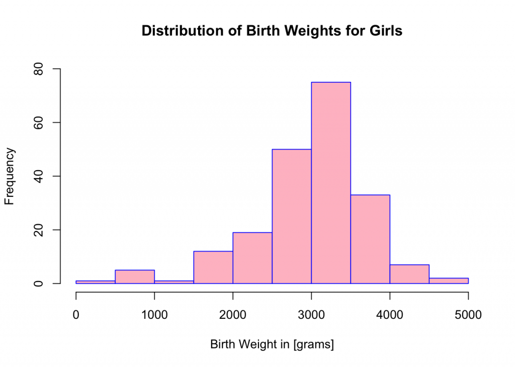
detach(girlD)Now: Select all rows from BirthsD data set that pertain to boys’ births and include all variables, (columns).
Start by naming this subset boyD, (boys’ data).
boyD <-BirthsD[GENDER..1.M. == "1", ]
attach(boyD)
## The following objects are masked from BirthsD:
##
## ADMITTED, BIRTH.WEIGHT, DISCHARGED, FACILITY, GENDER..1.M.,
## INSURANCE, LENGTH.OF.STAY, TOTAL.CHARGEShead(boyD,3)## FACILITY INSURANCE GENDER..1.M.
## 2 Albany Medical Center Hospital Blue Cross 1
## 4 Albany Medical Center Hospital Insurance Company 1
## 5 Albany Medical Center Hospital Insurance Company 1
## LENGTH.OF.STAY ADMITTED DISCHARGED BIRTH.WEIGHT TOTAL.CHARGES
## 2 2 FRI SUN 3900 3632.5
## 4 5 MON SAT 2800 8536.5
## 5 2 FRI SUN 3700 3632.5summary(BIRTH.WEIGHT)## Min. 1st Qu. Median Mean 3rd Qu. Max.
## 300 2900 3400 3273 3650 4900Create a frequency table for Boys’ birth weights.
BIRTH.WEIGHT.cut <-cut(BIRTH.WEIGHT,breaks)
BIRTH.WEIGHT.freq <-table(BIRTH.WEIGHT.cut)
transform(BIRTH.WEIGHT.freq)
## BIRTH.WEIGHT.cut Freq
## 1 (0,500] 1
## 2 (500,1e+03] 2
## 3 (1e+03,1.5e+03] 2
## 4 (1.5e+03,2e+03] 5
## 5 (2e+03,2.5e+03] 8
## 6 (2.5e+03,3e+03] 39
## 7 (3e+03,3.5e+03] 69
## 8 (3.5e+03,4e+03] 57
## 9 (4e+03,4.5e+03] 10
## 10 (4.5e+03,5e+03] 2Create a histogram of birth weights for boys data subset using breaks and hist command.
breaks<-seq(0,5000,by=500)
hist(BIRTH.WEIGHT, xlab = "Birth Weight in [grams]", ylab="Frequency",ylim=c(0,80),main="Distribution of Birth Weights for Boys", col="blue",border="yellow")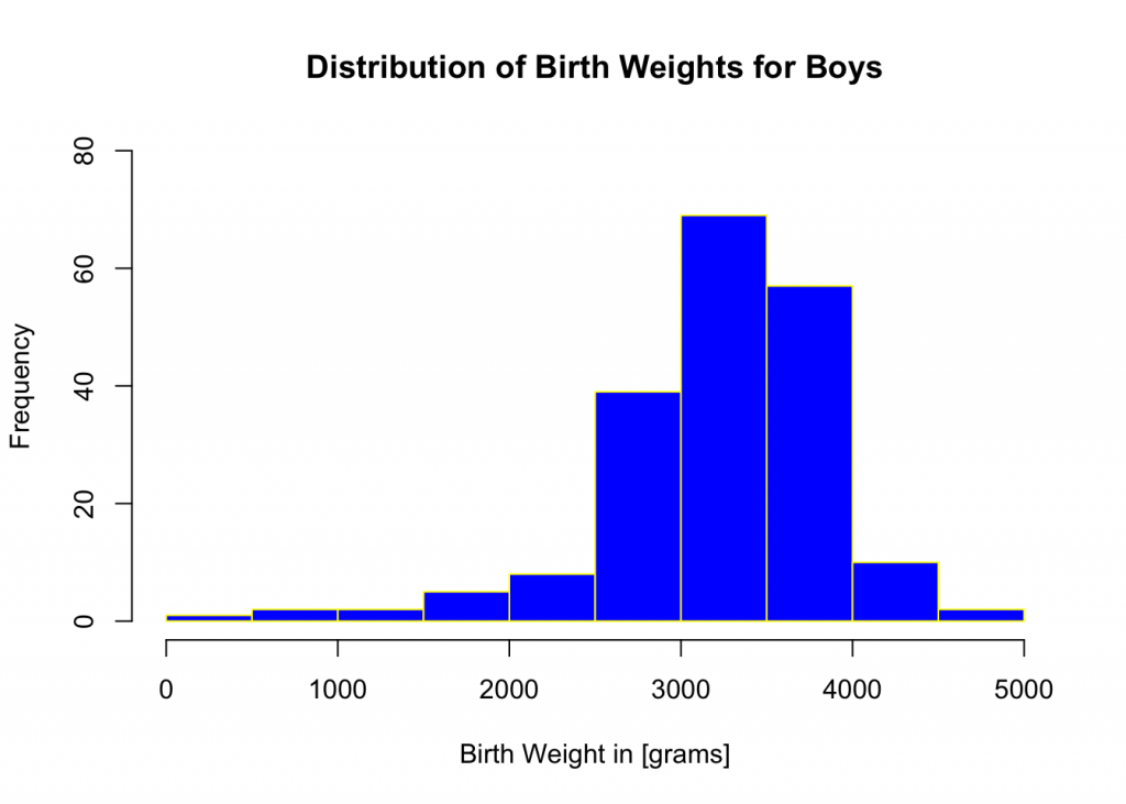
detach(boyD)Extra Credit Assignment
1. Use parts of the above syntax and create two box-and-whisker plots, (one for each gender), describe variability in each subset, and compare variability between genders.
2. Write a report using any word-processing program. Use full and complete sentences; remember to include numerical and graphical summaries in your report. In addition, attach R printout with input/output.
- Data Set 4: extracted from M. F Triola, Essentials of Statistics Sixth Edition, Pearson↩
Recent Comments