Five fair dice were rolled once and the proportion of ODD outcomes was observed.

Example 1

x <-sample(1:6,5,replace = TRUE); x

## [1] 5 2 2 5 4

What is the proportion of ODD outcomes?

y <- x %% 2;y

## [1] 1 0 0 1 0

prop <-sum(y)/length(x);prop

## [1] 0.4

Example 2 (Simulation)

Replicate 100,000 five-dice rolls and record the proportion of ODD numbers for each roll.

five.dice <- function() {
  dice <-sample(1:6,5, replace = TRUE)
  return(sum(dice %% 2)/length(dice))
}
sim1 <-replicate(100000, five.dice())

Here are the first six recorded proportions of ODD outcomes.

head(sim1)

## [1] 0.2 0.6 0.4 0.6 0.2 1.0

Table of Proportions of ODD outcomes from 100,000 simulated rolls

transform(table(sim1))

##   sim1  Freq
## 1    0  3065
## 2  0.2 15541
## 3  0.4 31303
## 4  0.6 31434
## 5  0.8 15626
## 6    1  3031

Histogram of Proportions of ODD Outcomes

breaks <-seq(-0.1,1.1,by=0.2)
hist(sim1,breaks, col="red", border = "green",xlab="Proportion of ODD Numbers",ylab="Frequency", main = "Sampling Distribution of Sample Proportion")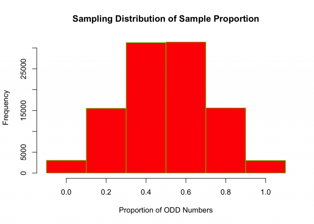

Finally, the mean proportion of simulated proportions is equal to:

mean(sim1)

## [1] 0.500216

Ponder on the following: a) shape of the sampling distribution of the sample proportion
b) the mean proportion of the sample proportion
c) proportion of ODD outcomes when rolling a fair die once
d) writing a simulation like the one above regarding the proportion of EVEN outcomes in 100,000 rolls of five-fair dice.