The Normal Distribution

Here is the Standard Normal Distribution Density Curve is also known as the Bell Curve.

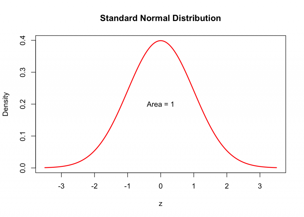
How do we find the area under the Standard Normal Density Curve?

Example 1

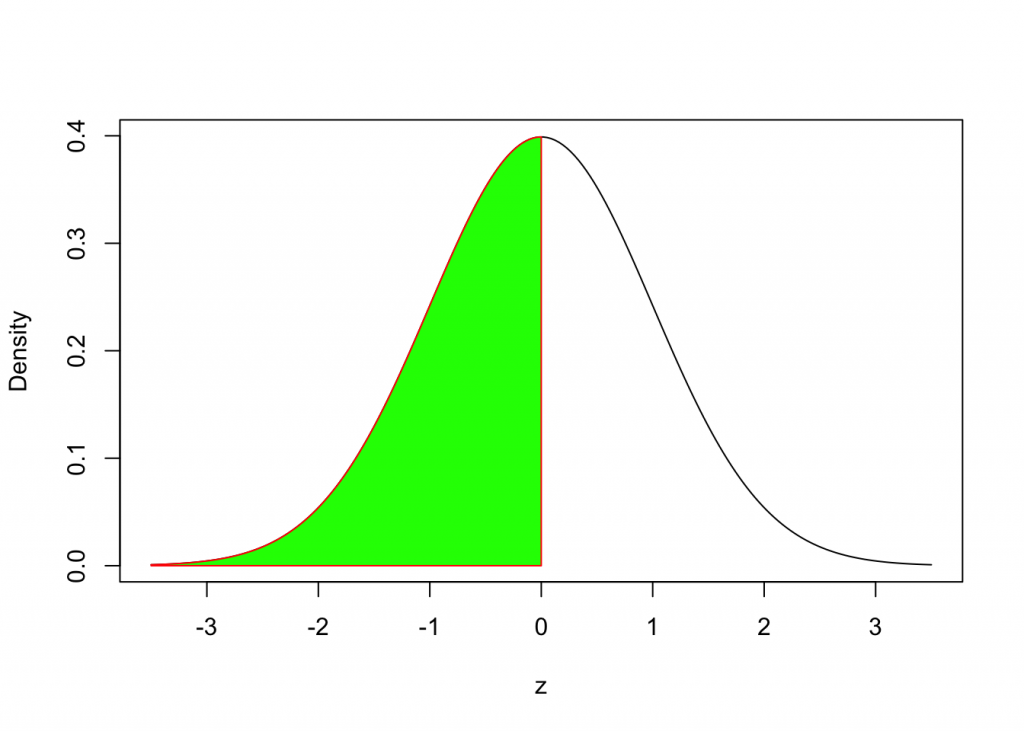
We will use the following syntax:

pnorm(0,mean=0,sd=1)

## [1] 0.5

Example 2

How do we find the area under the Standard Normal Density Curve to the left of z = 1.25?

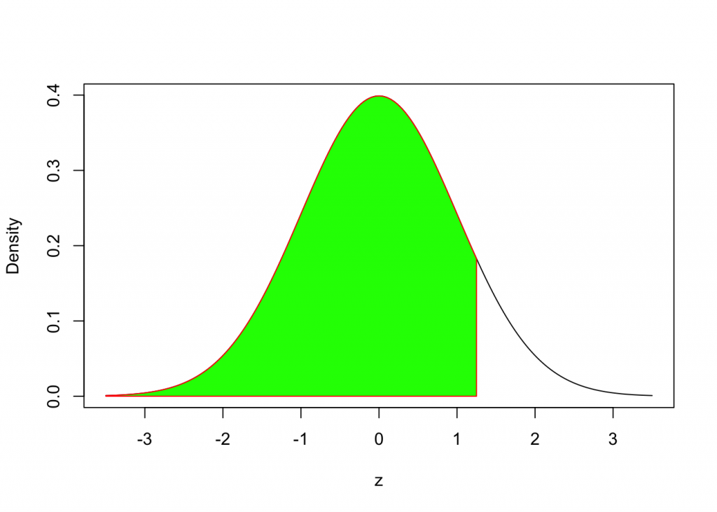
pnorm(1.25, mean=0,sd=1)

## [1] 0.8943502

Example 3

How do we find the area under the Standard Normal Density Curve to the right of z = 1.5?

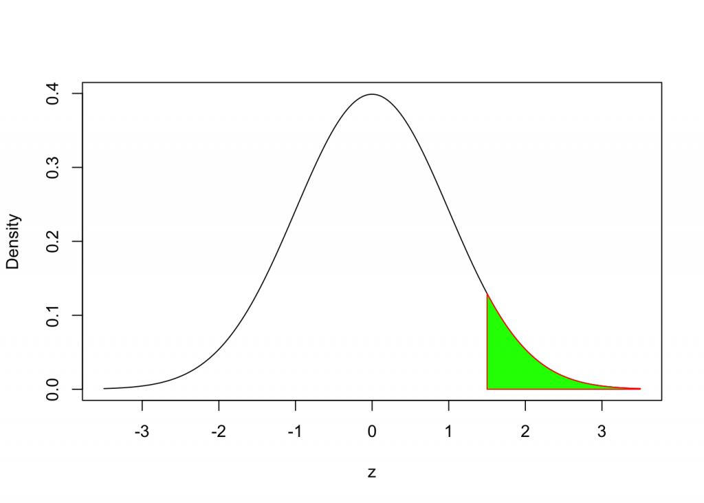
We can use the following syntax:

1 - pnorm(1.5, mean=0, sd=1)

## [1] 0.0668072

Alternatively the code below

pnorm(1.5, mean=0, sd = 1, lower.tail = FALSE)

## [1] 0.0668072

Example 4

How do we determine the area under the Standard Normal Curve between two z-values, (eg. z = -1.25 and z = 1.25)?

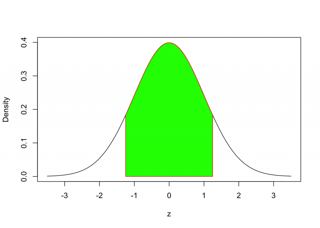
We can calculate the difference of two areas as follows:

pnorm(1.25, mean = 0, sd = 1) - pnorm(-1.25, mean = 0, sd = 1)

## [1] 0.7887005

Summary:

The following code pnorm(z, mean, sd) provides the area under the Standard Normal Density Curve to the left of z-value.

Assignment 2

The bone density test scores follow standard normal distribution for children, healthy premenopausal young women, and men under 50. Assume that a randomly selected person is subjected to a bone density test. Find the probability that this person has a score:

1. z < -2.5
2. -2.5 < z < -1
3. z > -1.

Note: For each part: a, b and c include distribution statement, density curve with shaded area. Also, use a full and complete sentence as the answer to a, b, and c part.
link