Tutorial/Extra Credit Assignment

How to partition Births Data Set¹ by gender?

How to create a histogram of Birth Weight Data Set for each gender?

Upload data set by using the following syntax:

BirthsD <-read.csv(file.choose(),header =TRUE)

attach(BirthsD)
head(BirthsD,3)

##                         FACILITY         INSURANCE GENDER..1.M.
## 1 Albany Medical Center Hospital Insurance Company            0
## 2 Albany Medical Center Hospital        Blue Cross            1
## 3 Albany Medical Center Hospital        Blue Cross            0
##   LENGTH.OF.STAY ADMITTED DISCHARGED BIRTH.WEIGHT TOTAL.CHARGES
## 1              2      FRI        SUN         3500       13985.7
## 2              2      FRI        SUN         3900        3632.5
## 3             36      WED        THU          800      359091.0

Select all rows from the BirthsD data set that pertain to girls’ births and include all variables, (columns).

Start by naming this subset girlD, (girls data).

girlD <-BirthsD[GENDER..1.M. == "0",]
attach(girlD)

## The following objects are masked from BirthsD:
## 
##     ADMITTED, BIRTH.WEIGHT, DISCHARGED, FACILITY, GENDER..1.M.,
##     INSURANCE, LENGTH.OF.STAY, TOTAL.CHARGES

head(girlD)

##                          FACILITY         INSURANCE GENDER..1.M.
## 1  Albany Medical Center Hospital Insurance Company            0
## 3  Albany Medical Center Hospital        Blue Cross            0
## 6  Albany Medical Center Hospital        Blue Cross            0
## 7  Albany Medical Center Hospital          Medicaid            0
## 9  Albany Medical Center Hospital Insurance Company            0
## 13 Albany Medical Center Hospital Insurance Company            0
##    LENGTH.OF.STAY ADMITTED DISCHARGED BIRTH.WEIGHT TOTAL.CHARGES
## 1               2      FRI        SUN         3500       13985.7
## 3              36      WED        THU          800      359091.0
## 6               4      FRI        TUE         2400        6406.0
## 7               3      TUE        FRI         4200        4778.0
## 9               2      SAT        MON         3100        3860.0
## 13              4      SUN        THU         2000        6986.9

summary(BIRTH.WEIGHT)

##    Min. 1st Qu.  Median    Mean 3rd Qu.    Max. 
##     300    2700    3100    3037    3500    4700

Create a frequency table for Girls’ birth weights.

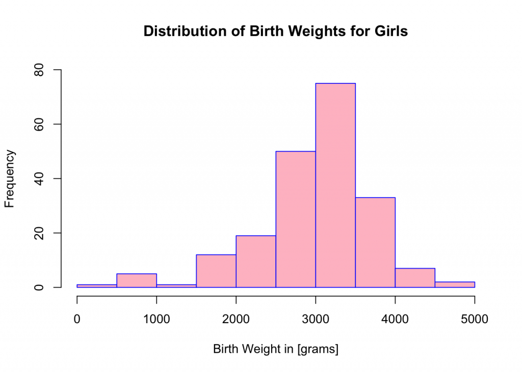
breaks <-seq(0,5000,by=500)
BIRTH.WEIGHT.cut <-cut(BIRTH.WEIGHT,breaks)
BIRTH.WEIGHT.freq <-table(BIRTH.WEIGHT.cut)
frequency.table <-transform(BIRTH.WEIGHT.freq)
frequency.table

##    BIRTH.WEIGHT.cut Freq
## 1           (0,500]    1
## 2       (500,1e+03]    5
## 3   (1e+03,1.5e+03]    1
## 4   (1.5e+03,2e+03]   12
## 5   (2e+03,2.5e+03]   19
## 6   (2.5e+03,3e+03]   50
## 7   (3e+03,3.5e+03]   75
## 8   (3.5e+03,4e+03]   33
## 9   (4e+03,4.5e+03]    7
## 10  (4.5e+03,5e+03]    2

Create a histogram of birth weights for girls’ data subset using breaks and hist command.

breaks<-seq(0,5000,by=500)
hist(BIRTH.WEIGHT, xlab = "Birth Weight in [grams]", ylab="Frequency",ylim=c(0,80),main="Distribution of Birth Weights for Girls", col="pink",border="blue")

detach(girlD)

Now: Select all rows from BirthsD data set that pertain to boys’ births and include all variables, (columns).

Start by naming this subset boyD, (boys’ data).

boyD <-BirthsD[GENDER..1.M. == "1", ]
attach(boyD)

## The following objects are masked from BirthsD:
## 
##     ADMITTED, BIRTH.WEIGHT, DISCHARGED, FACILITY, GENDER..1.M.,
##     INSURANCE, LENGTH.OF.STAY, TOTAL.CHARGES

head(boyD,3)

##                         FACILITY         INSURANCE GENDER..1.M.
## 2 Albany Medical Center Hospital        Blue Cross            1
## 4 Albany Medical Center Hospital Insurance Company            1
## 5 Albany Medical Center Hospital Insurance Company            1
##   LENGTH.OF.STAY ADMITTED DISCHARGED BIRTH.WEIGHT TOTAL.CHARGES
## 2              2      FRI        SUN         3900        3632.5
## 4              5      MON        SAT         2800        8536.5
## 5              2      FRI        SUN         3700        3632.5

summary(BIRTH.WEIGHT)

##    Min. 1st Qu.  Median    Mean 3rd Qu.    Max. 
##     300    2900    3400    3273    3650    4900

Create a frequency table for Boys’ birth weights.

BIRTH.WEIGHT.cut <-cut(BIRTH.WEIGHT,breaks)
BIRTH.WEIGHT.freq <-table(BIRTH.WEIGHT.cut)
transform(BIRTH.WEIGHT.freq)

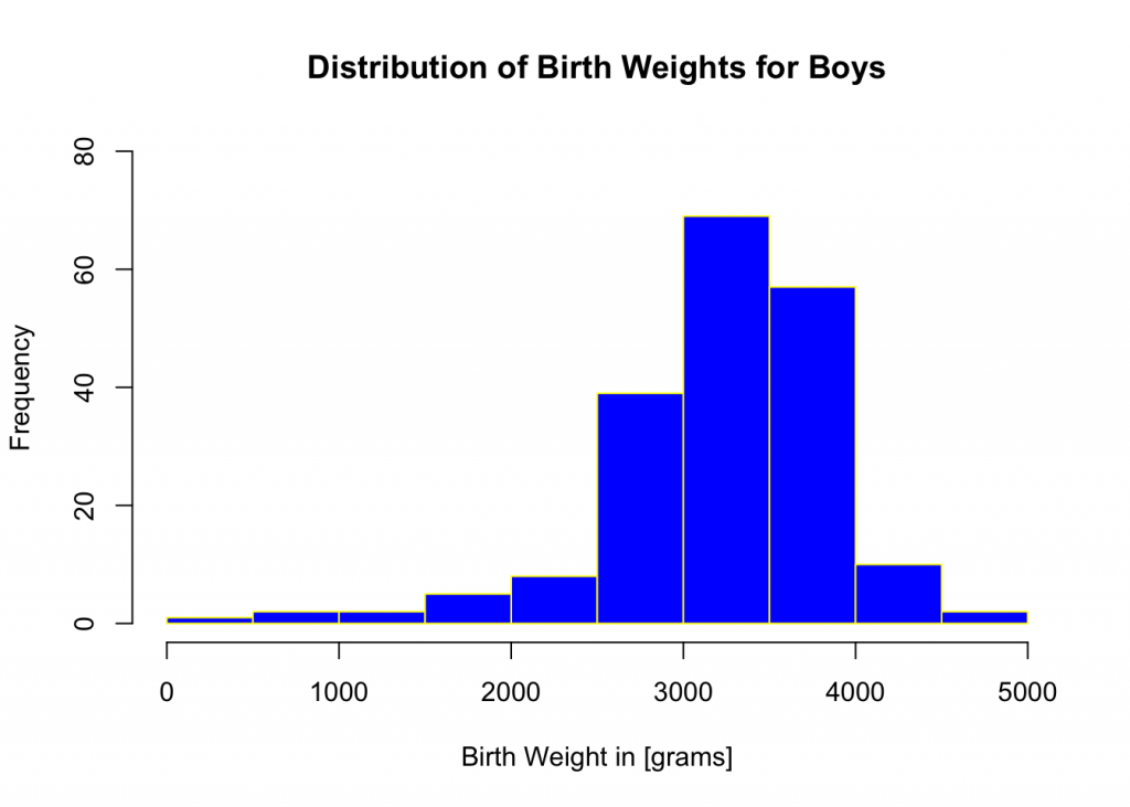
##    BIRTH.WEIGHT.cut Freq
## 1           (0,500]    1
## 2       (500,1e+03]    2
## 3   (1e+03,1.5e+03]    2
## 4   (1.5e+03,2e+03]    5
## 5   (2e+03,2.5e+03]    8
## 6   (2.5e+03,3e+03]   39
## 7   (3e+03,3.5e+03]   69
## 8   (3.5e+03,4e+03]   57
## 9   (4e+03,4.5e+03]   10
## 10  (4.5e+03,5e+03]    2

Create a histogram of birth weights for boys data subset using breaks and hist command.

breaks<-seq(0,5000,by=500)
hist(BIRTH.WEIGHT, xlab = "Birth Weight in [grams]", ylab="Frequency",ylim=c(0,80),main="Distribution of Birth Weights for Boys", col="blue",border="yellow")

detach(boyD)

Extra Credit Assignment

1. Use parts of the above syntax and create two box-and-whisker plots, (one for each gender), describe variability in each subset, and compare variability between genders.

2. Write a report using any word-processing program. Use full and complete sentences; remember to include numerical and graphical summaries in your report. In addition, attach R printout with input/output.

---

1. Data Set 4: extracted from M. F Triola, Essentials of Statistics Sixth Edition, Pearson↩